Welcome to the official home of the WrightMap package
WrightMap Tutorial 5
More Flexibility using the person and item side functions
Introduction
Version 1.2 of the WrightMap package allows you to directly access the functions used for drawing the person and item sides of the map in order to allow more flexible item person maps. The parts can be put together on the same plot using the split.screen function.
Calling the functions
Let’s start by installing and loading the latest version of the package from CRAN.
install.packages('WrightMap')
library(WrightMap)
And set up some item data.
set.seed(2020)
items.loc <- sort( rnorm( 20))
  thresholds <- data.frame(
    l1 = items.loc - 0.5 ,
    l2 = items.loc - 0.25,
    l3 = items.loc + 0.25,
    l4 = items.loc + 0.5)
We can draw a simple item map by calling one of the item side functions. Currently there are three: itemModern , itemClassic , and itemHist .
The itemModern function is the default called by wrightMap .
itemModern(thresholds)

The itemClassic function creates item sides inspired by text-based Wright Maps.
itemClassic(thresholds)

Finally, the itemHist function plots the items as a histogram.
itemHist(thresholds)

Similarly, the person side functions allow you to graph the person parameters. There are two, personHist and personDens .
## Mock results
  multi.proficiency <- data.frame(
    d1 = rnorm(1000, mean =  -0.5, sd = .5),
    d2 = rnorm(1000, mean =   0.0, sd = 1),
    d3 = rnorm(1000, mean =  +0.5, sd = 1),
    d4 = rnorm(1000, mean =   0.0, sd = .5),
    d5 = rnorm(1000, mean =  -0.5, sd = .75))
personHist(multi.proficiency)

personDens(multi.proficiency)

To use these plots in a Wright Map, use the item.side and person.side parameters.
wrightMap(multi.proficiency,thresholds,item.side = itemClassic, item.prop = 0.5,person.side = personDens)

Use with CQmodel: The personData and itemData functions
The person side and item side functions are expecting data in the form of matrices. They do not recognize CQmodel objects. When a CQModel object is sent to wrightMap , it first extracts the necessary data, and then sends the data to the plotting functions. In 1.2, the data processing functions have also been made directly accessible to users in the form of the personData and itemData functions. These are fast ways to pull the data out of a CQmodel object in such a way that it is ready to be sent to wrightMap or any of the item and person plotting functions.
The personData function is very simple. It can take either a CQmodel object or a string containing the name of a ConQuest person parameter file. It extracts the person estimates as a matrix.
fpath <- system.file("extdata", package="WrightMap")
model1 <- CQmodel(file.path(fpath,"ex7a.eap"), file.path(fpath,"ex7a.shw"))

head(model1$p.est)

##   casenum est (d1) error (d1) pop (d1) est (d2) error (d2) pop (d2)
## 1       1  1.37364    0.70308  0.60309  1.73654    0.60556  0.52928
## 2       2 -0.17097    0.64866  0.66216  0.75620    0.54852  0.61379
## 3       3  0.46677    0.64837  0.66246  0.85146    0.55129  0.60987
## 4       4  0.67448    0.66017  0.65006  1.16098    0.56368  0.59214
## 5       5  0.89717    0.67704  0.63195  1.49079    0.58539  0.56012
## 6       6  1.64704    0.72529  0.57762  2.11784    0.62916  0.49188

m1.person <- personData(model1)

head(m1.person)
##         d1      d2
## 1  1.37364 1.73654
## 2 -0.17097 0.75620
## 3  0.46677 0.85146
## 4  0.67448 1.16098
## 5  0.89717 1.49079
## 6  1.64704 2.11784
personHist(m1.person,dim.lab.side = 1)

The itemData function uses the GIN table (Thurstonian thresholds) if it is there, and otherwise tries to create delta parameters out of the RMP tables. You can also specify tables to use as items, steps, and interactions, and it will add them together appropriately to create delta parameters.
model2 <- CQmodel(file.path(fpath,"ex4a.mle"), file.path(fpath,"ex4a.shw"))
names(model2$RMP)

## [1] "rater"                     "topic"
## [3] "criteria"                  "rater*topic"
## [5] "rater*criteria"            "topic*criteria"
## [7] "rater*topic*criteria*step"
m2.item <- itemData(model2,item.table = "topic", interactions = "rater*topic", step.table = "rater")

itemModern(m2.item)

See Tutorial 4 for details on specifying tables from CQmodel objects.
Having these data functions pulled out also makes it easier to combine parameters from different models onto a single plot (when appropriate).
wrightMap(m1.person,m2.item)

Putting it all together with split.screen
By calling these functions directly and using, we can make Wright Maps with other arrangements of persons and items. The item side functions can be combined using any of the base graphics options for combining plots (layout, par(mfrow)), but the person side functions are based on split.screen , which is incompatible with those options. We will be combining item and person maps, so we need to use split.screen .
The first step of combining these functions is to set up the screens. Details for screen functions are in the documentation for split.screen . The function takes as a parameter a 4-column matrix, in which each row is a screen, and the columns represent the left, bottom, right, and top of the screens respectively. Each value is expressed as a number from 0 to 1, where 0 is the left/bottom of the current device and 1 is the right/top.
To make a Wright Map with the items on the left and the persons on the right, we will set up two screens, with 80% of the width on the left and 20% on the right.
split.screen(figs = matrix(c(0,.8,0,1
                            ,.8,1,0,1),ncol = 4, byrow = TRUE))
Next, we’ll draw the item side. IMPORTANT NOTE: Make sure to explicitly set the yRange variable when combining plots to ensure they are on the same scale. We can also adjust some of the other parameters to work better with a left-side item plot. We’ll move the logit axis to the left with the show.axis.logit parameter, and set the righthand outer margin to 2 to give us a space between the plots.
itemModern(thresholds, yRange = c(-3,4), show.axis.logits = "L", oma = c(0,0,0,2))

# We can also add a title at this time.

mtext("Wright Map", side = 3, font = 2, line = 1)
Finally, we will move to screen 2 and draw the person side. This plot will be adjusted to move the persons label and remove the axis.
screen(2)


personHist(multi.proficiency, axis.persons = "",yRange = c(-3,4)
    , axis.logits = "Persons", show.axis.logits = FALSE)
The last thing to do is to close all the screens to prevent them from getting in the way of any future plotting.
close.screen(all.screens = TRUE)
Here is the complete plot:
split.screen(figs = matrix(c(0,.8,0,1,.8,1,0,1),ncol = 4, byrow = TRUE))

itemModern(thresholds, yRange = c(-3,4), show.axis.logits = "L", oma = c(0,0,0,2))
mtext("Wright Map", side = 3, font = 2, line = 1)

screen(2)

personHist(multi.proficiency, axis.persons = "",yRange = c(-3,4)
    , axis.logits = "Persons", show.axis.logits = FALSE)

close.screen(all.screens = TRUE)

Countless arrangements are possible. As one last example, here are two ways to put two dimensions put side by side in separate Wright Maps.
Explicitly splitting the device into four screens:
d1 = rnorm(1000, mean =  -0.5, sd = 1)
d2 = rnorm(1000, mean =   0.0, sd = 1)

dim1.diff <- rnorm(5)
dim2.diff <- rnorm(5)

split.screen(figs = matrix(c(  0,.09,0,1,
                             .11,.58,0,1,
                              .5,.59,0,1,
                             .51,  1,0,1), ncol = 4, byrow = TRUE))

    personDens(d1,yRange = c(-3,3),show.axis.logits = FALSE, axis.logits = "")

screen(2)
    itemModern(dim1.diff,yRange = c(-3,3),show.axis.logits = FALSE)
    mtext("Wright Map", side = 3, font = 2, line = 1)

screen(3)
    personDens(d2,yRange = c(-3,3),show.axis.logits = FALSE
        , axis.logits = ""
        , axis.persons = "",dim.names = "Dim2")

screen(4)
    itemModern(dim2.diff,yRange = c(-3,3),show.axis.logits = FALSE
        , label.items = paste("Item",6:10))

close.screen(all.screens = TRUE)
Splitting the device into two screens with a Wright Map on each:
split.screen(figs = matrix(c( 0,.5,0,1,
                             .5, 1,0,1), ncol = 4, byrow = TRUE))

    wrightMap(d1,dim1.diff,person.side = personDens,show.axis.logits = FALSE)

screen(2)
    wrightMap(d2,dim2.diff,person.side = personDens,show.axis.logits = FALSE)

close.screen(all.screens = TRUE)

WrightMap Tutorial 4
Using Conquest Output and Making Thresholds
Updated Fri 24-Apr-2020
Intro
In this part of the tutorial, we’ll show how to load ConQuest output to make a CQmodel object and then WrightMaps. We’ll also show how to turn deltas into thresholds. All the example files here are available in the /inst/extdata folder of our github site. If you download the latest version of the package, they should be in a folder called /extdata wherever your R packages are stored. You can set this folder as your working directory with setwd() or use the system.file() command—as in the next set of examples—to run them.
Making the model
Let’s load a model. The first parameter should be the name of the person estimates file, while the second should be the name of the show file. Both are necessary for creating Wright maps (although the CQmodel function will run fine with only one or the other, provided that they are properly passed).
We start by defining a path to the WrightMap example files.
fpath <- system.file("extdata", package="WrightMap")
And we load the example output.
model1 <- CQmodel(p.est = file.path(fpath,"ex2.eap"), show = file.path(fpath,"ex2.SHW"))
This (model1) is a CQmodel object. Enter the name of the object to see the names of all the tables & information stored within this object.
model1

##
## ConQuest Output Summary:
## ========================
## Partial Credit Analysis
##
## The item model: item+item*step
## 1 dimension
## 582 participants
## Deviance: 9272.597 (21 parameters)
##
## Additional information available:
## Summary of estimation: $SOE
## Response model parameter estimates: $RMP
## Regression coefficients: $reg.coef
## Variances: $variances
## Reliabilities: $rel.coef
## GIN tables (thresholds): $GIN
## EAP table: $p.est
## Additional details: $run.details
Type the name of any of these tables to see the information stored there.
model1$SOE

##
## Summary of estimation
##
## Estimation method: Gauss-Hermite Quadrature with 15 nodes
## Assumed population distribution: Gaussian
## Constraint: DEFAULT
##
## Termination criteria:
##       1000 iterations
##       0.0001 change in parameters
##       0.0001 change in deviance
##       100 iterations without a deviance improvement
##       10 Newton steps in M-step
## Estimation terminated after 27 iterations because the deviance convergence criteria was reached.
##
## Random number generation seed: 1
## 2000 nodes used for drawing 5 plausible values
## 200 nodes used when computing fit
## Value for obtaining finite MLEs for zero/perfects: 0.3
model1$equation

## [1] "item+item*step"
model1$reg.coef

##                CONSTANT
## Main dimension    0.972
## S. errors         0.062
model1$rel.coef

## MLE Person separation RELIABILITY
## Main dimension NA
##
## WLE Person separation RELIABILITY
## Main dimension NA
##
## EAP/PV RELIABILITY
## Main dimension 0.813

```R
model1$variances

##            errors
## [1,] 2.162     NA
The most relevant for our purposes are the RMP , GIN , and p.est tables. The RMP tables contain the Response Model Parameters. These are item parameters. Typing model1$RMP would display them, but they’re a little long, so I’m just going to ask for the names and then show the first few rows of each table.
`names(model1$RMP)

## [1] "item"      "item*step"
For this model, the RMPs have item and item*step parameters. We could add these to get the deltas. Let’s see what the tables look like.
head(model1$RMP$item)

##   n_item item    est error U.fit U.Low U.High  U.T W.fit W.Low W.High  W.T
## 1      1    1  0.753 0.055  1.11  0.88   1.12  1.8  1.10  0.89   1.11  1.8
## 2      2    2  1.068 0.053  1.41  0.88   1.12  6.0  1.37  0.89   1.11  6.0
## 3      3    3 -0.524 0.058  0.82  0.88   1.12 -3.2  0.87  0.88   1.12 -2.3
## 4      4    4 -1.174 0.060  0.76  0.88   1.12 -4.3  0.85  0.88   1.12 -2.7
## 5      5    5 -0.389 0.057  0.95  0.88   1.12 -0.9  0.95  0.89   1.11 -0.9
## 6      6    6  0.067 0.055  1.03  0.88   1.12  0.6  1.02  0.89   1.11  0.3
head(model1$RMP$"item*step")

##   n_item item step    est error U.fit U.Low U.High  U.T W.fit W.Low W.High  W.T
## 1      1    1    0     NA    NA  2.03  0.88   1.12 13.3  1.18  0.89   1.11  3.0
## 2      1    1    1 -1.129 0.090  0.99  0.88   1.12 -0.1  1.00  0.95   1.05  0.0
## 3      1    1    2  1.129    NA  0.80  0.88   1.12 -3.5  0.95  0.89   1.11 -0.9
## 4      2    2    0     NA    NA  2.25  0.88   1.12 15.4  1.40  0.90   1.10  7.1
## 5      2    2    1 -0.626 0.093  1.04  0.88   1.12  0.7  1.04  0.94   1.06  1.3
## 6      2    2    2  0.626    NA  1.08  0.88   1.12  1.2  1.08  0.89   1.11  1.4
Let’s look at a more complicated example.
model2

## [1] "rater+topic+criteria+rater*topic+rater*criteria+topic*criteria+rater*topic*criteria*step"
names(model2$RMP)

## [1] "rater"                     "topic"
## [3] "criteria"                  "rater*topic"
## [5] "rater*criteria"            "topic*criteria"
## [7] "rater*topic*criteria*step"
head(model2$RMP$"rater*topic*criteria*step")

##   n_rater    rater n_topic topic n_criteria criteria step    est error U.fit U.Low U.High  U.T W.fit W.Low W.High W.T
## 1       1      Amy       1 Sport          1 spelling    1     NA    NA  0.43  0.70   1.30 -4.7  0.99  0.00   2.00 0.1
## 2       1      Amy       1 Sport          1 spelling    2  0.299 0.398  1.34  0.70   1.30  2.1  1.05  0.42   1.58 0.3
## 3       1      Amy       1 Sport          1 spelling    3 -0.299    NA  1.28  0.70   1.30  1.7  1.05  0.51   1.49 0.3
## 4       2 Beverely       1 Sport          1 spelling    0     NA    NA  0.41  0.74   1.26 -5.8  1.47  0.00   2.09 0.9
## 5       2 Beverely       1 Sport          1 spelling    1 -0.184 0.491  3.23  0.74   1.26 10.9  0.95  0.30   1.70 0.0
## 6       2 Beverely       1 Sport          1 spelling    2  0.051 0.461  0.87  0.74   1.26 -1.0  1.30  0.62   1.38 1.5
The GIN tables show the threshold parameters.
model1$GIN

##           [,1]  [,2]
## Item_1  -0.469 1.977
## Item_2   0.234 1.906
## Item_3  -1.789 0.742
## Item_4  -2.688 0.336
## Item_5  -1.656 0.883
## Item_6  -1.063 1.195
## Item_7  -1.969 1.047
## Item_8  -1.617 1.289
## Item_9  -0.957 1.508
## Item_10 -0.992 2.094
model2$GIN

## $Amy
## $Amy$Sport
##              [,1]   [,2]   [,3]
## spelling  -31.996 -1.976 -1.250
## coherence  -1.447 -1.446 -1.209
## structure  -2.247 -0.911 -0.172
## grammar    -0.885 -0.773 -0.107
## content    -0.486  0.104  0.627
##
## $Amy$Family
##              [,1]   [,2]   [,3]
## spelling  -31.996 -2.516 -0.912
## coherence  -1.401 -1.280 -1.103
## structure  -1.966 -1.260 -0.294
## grammar    -1.069 -0.380 -0.106
## content    -0.728 -0.012  0.950
##
## $Amy$Work
##             [,1]   [,2]   [,3]
## spelling  -2.055 -2.051 -1.128
## coherence -1.515 -1.320 -0.862
## structure -1.402 -1.158 -0.631
## grammar   -0.816 -0.550  0.122
## content   -0.430  0.212  0.762
##
## $Amy$School
##              [,1]   [,2]   [,3]
## spelling  -31.996 -2.059 -0.997
## coherence  -1.403 -1.402 -0.999
## structure  -1.629 -1.148 -0.462
## grammar    -0.967 -0.421  0.070
## content    -0.782 -0.027  1.121
##
##
## $Beverely
## $Beverely$Sport
##             [,1]   [,2]   [,3]
## spelling  -2.054 -1.339 -0.663
## coherence -1.751 -1.129 -0.674
## structure -1.042 -0.437  0.013
## grammar   -0.502 -0.082  0.529
## content   -0.253  0.613  1.184
##
## $Beverely$Family
##              [,1]   [,2]   [,3]
## spelling  -31.996 -2.264 -0.718
## coherence  -1.524 -1.357 -0.684
## structure  -1.326 -0.577  0.164
## grammar    -0.796  0.118  0.599
## content    -0.469  0.690  1.230
##
## $Beverely$Work
##             [,1]   [,2]   [,3]
## spelling  -2.366 -1.465 -0.672
## coherence -1.388 -1.088 -0.925
## structure -1.115 -0.621  0.197
## grammar   -0.345  0.045  0.495
## content   -0.212  0.482  1.282
##
## $Beverely$School
##             [,1]   [,2]   [,3]
## spelling  -1.826 -1.611 -0.873
## coherence -1.632 -1.222 -0.794
## structure -1.270 -0.865  0.321
## grammar   -0.491 -0.037  0.413
## content   -0.361  0.449  1.137
##
##
## $Colin
## $Colin$Sport
##             [,1]   [,2]  [,3]
## spelling  -1.660 -0.685 0.564
## coherence -0.612 -0.168 0.362
## structure -0.485  0.519 1.512
## grammar    0.611  1.275 1.698
## content    1.037  1.853 2.343
##
## $Colin$Family
##             [,1]   [,2]   [,3]
## spelling  -1.477 -0.677 -0.022
## coherence -0.441 -0.277  0.332
## structure -0.318  0.265  1.299
## grammar    0.361  1.252  1.839
## content    1.009  1.683  2.374
##
## $Colin$Work
##             [,1]   [,2]  [,3]
## spelling  -1.697 -1.002 0.089
## coherence -0.654 -0.105 0.192
## structure -0.502  0.502 1.205
## grammar    0.662  1.218 1.573
## content    0.766  1.806 2.357
##
## $Colin$School
##             [,1]   [,2]  [,3]
## spelling  -1.595 -0.788 0.095
## coherence -0.629 -0.389 0.123
## structure -0.470  0.122 1.237
## grammar    0.385  1.010 1.679
## content    0.698  1.520 2.310
##
##
## $David
## $David$Sport
##             [,1]   [,2]  [,3]
## spelling  -1.405 -0.482 0.412
## coherence -0.357  0.136 0.581
## structure  0.023  0.724 1.811
## grammar    0.714  1.454 1.959
## content    1.256  2.031 2.912
##
## $David$Family
##             [,1]   [,2]  [,3]
## spelling  -1.271 -0.404 0.741
## coherence  0.028  0.415 0.977
## structure  0.474  1.069 1.756
## grammar    1.177  1.733 2.085
## content    1.284  2.169 3.596
##
## $David$Work
##             [,1]   [,2]  [,3]
## spelling  -1.378 -0.587 0.498
## coherence -0.119  0.260 0.795
## structure  0.173  1.003 1.885
## grammar    1.199  1.592 2.008
## content    1.437  2.174 3.117
##
## $David$School
##             [,1]   [,2]  [,3]
## spelling  -0.815 -0.330 0.424
## coherence  0.062  0.293 0.805
## structure  0.295  1.012 1.955
## grammar    1.035  1.642 2.260
## content    1.312  2.107 3.407
Finally, the p.est table shows person parameters.
head(model1$p.est)  ##EAPs

##   casenum est (d1) error (d1) pop (d1)
## 1       1 -0.08240    0.50495  0.88205
## 2       2  1.75925    0.55966  0.85510
## 3       3  0.16483    0.49122  0.88838
## 4       4  3.57343    0.82692  0.68367
## 5       5 -0.62303    0.52908  0.87051
## 6       6  0.16483    0.49122  0.88838
head(model2$p.est)  ##MLEs

##   casenum sscore (d1) max (d1) est (d1) error (d1)
## 1       1          23       60 -0.49687    0.25349
## 2       2          36       60  0.69311    0.26051
## 3       3          24       60 -0.26371    0.26378
## 4       4          52       60  1.85869    0.37825
## 5       5          47       60  1.91466    0.28843
## 6       6          47       60  0.53122    0.28348
CQmodel, meet wrightMap
Ok, we have person parameters and item parameters: Let’s make a Wright Map
wrightMap(model1)
## Using GIN table for threshold parameters`

The above uses the GIN table as thresholds. But you may want to use RMP tables. For example, if you have an item table and an item _step table, you might want to combine them to make deltas. You could do this yourself, but you could also let the `make.deltas` function do it for you. This function reshapes the item_ step parameters, checks the item numbers to see if there are any dichotomous items, and then adds the steps and items. This can be especially useful if you didn’t get a GIN table from ConQuest (see below).
```R
model3 <- CQmodel(file.path(fpath,"ex2a.eap"), file.path(fpath,"ex2a.shw"))
model3$GIN
## NULL
model3$equation

## [1] "item+item*step"
This model has no GIN table, but it does have item and item*step tables. The make.deltas function will read the model equation and look for the appropriate tables.
make.deltas(model3)

##                    1      2      3
## Earth shape   -0.961 -0.493     NA
## Earth pictu.. -0.650  0.256  2.704
## Falling off   -1.416  1.969  1.265
## What is Sun   -0.959  1.343     NA
## Moonshine      0.157 -0.482 -0.128
## Moon and ni.. -0.635  0.861     NA
## Night and d..  0.157 -0.075 -0.739
## Breathe on ..  0.657  1.152 -3.558
When sent a model with no GIN table, wrightMap will automatically send it to make.deltas without the user having to ask.
wrightMap(model3, label.items.row = 2)

The make.deltas function can also handle rating scale models.
model4

## NULL
model4$equation

## [1] "item+step"
This rating scale model again has no GIN table (always the first thing wrightMap looks for) so we’ll need to make deltas.
make.deltas(model4)

##                    1     2
## Curriculum .. -0.468 1.900
## Not Until E.. -0.123 2.245
## Financial R.. -1.743 0.625
## Staff Commi.. -2.230 0.138
## Commitment .. -1.609 0.759
## Run for som.. -1.193 1.175
## Achievable .. -1.570 0.798
## Principals .. -1.317 1.051
## Parents sup.. -0.952 1.416
## Student mot.. -0.636 1.732
Or let wrightMap make them automatically.
wrightMap(model4, label.items.row = 2)

Specifying the tables
In the above examples, we let wrightMap decide what parameters to graph. WrightMap starts by looking for a GIN table. If it finds that, it assumes they are thresholds and graphs them accordingly. If there is no GIN table, it then sends the function to make.deltas , which will examine the model equation to see if it knows how to handle it. Make.deltas can handle equations of the form
A (e.g. item )
A + B (e.g. item + step [RSM])
A + A * B (e.g. item + item * step [PCM])
A + A * B + B (e.g item + item * gender + gender )
(It will also notice if there are minus signs rather than plus signs and react accordingly.)
But sometimes we may want something other than the default. Let’s look at model2 again.
model2$equation

## [1] "rater+topic+criteria+rater*topic+rater*criteria+topic*criteria+rater*topic*criteria*step"
Here’s the default Wright Map (we are adding the min.logit.pad correction because there are some very lo facet estimates), using the GIN table:
wrightMap(model2, min.logit.pad = -29)

## Using GIN table for threshold parameters

This doesn’t look great. Instead of showing all these estimates, we can specify a specific RMP table to use using the item.table parameter.
wrightMap(model2, item.table = "rater")

That shows just the rater parameters. Here’s just the topics.
wrightMap(model2, item.table = "topic")

What I really want, though, is to show the rater*topic estimates. For this, we can use the interactions and step.table parameters.
wrightMap(model2, item.table = "rater", interactions = "rater*topic"
	, step.table = "topic")

Switch the item and step names to graph it the other way:
wrightMap(model2, item.table = "topic", interactions = "rater*topic"
	, step.table = "rater")

You can leave out the interactions to have more of a rating scale-type model.
wrightMap(model2, item.table = "rater", step.table = "topic")

Or leave out the step table:
wrightMap(model2, item.table = "rater", interactions = "rater*topic")

Again, make.deltas is reading the model equation to decide whether to add or subtract. If, for some reason, you want to specify a different sign for one of the tables, you can use item.sign , step.sign , and inter.sign for that.
wrightMap(model2, item.table = "rater", interactions = "rater*topic"
	, step.table = "topic", step.sign = -1)

The last few examples might not make sense for this model, but are just to illustrate how the function works. Note that all three of these parameters must be the exact name of specific RMP tables, and you can’t specify an interactions table or a step table without also specifying an item table (although JUST an item table is fine). And if your model equation is more complicated than the ones specified above, you will have to either use a GIN table or specify in the function call which tables to use for what. A model of the form item + item * step + booklet , for example, will not run unless there is a GIN table or you have defined at least the item.table.
Making thresholds
So far, we’ve seen how to use the GIN table to graph thresholds, or the RMP tables to graph deltas. We have one use case left: Making thresholds out of those RMP-generated deltas. Coulter (Dan) Furr has provided a lovely function for exactly this purpose. The example below uses the model3 deltas, but you can send it any matrix with items as rows and steps as columns.
deltas <- make.deltas(model3)

deltas

##                    1      2      3
## Earth shape   -0.961 -0.493     NA
## Earth pictu.. -0.650  0.256  2.704
## Falling off   -1.416  1.969  1.265
## What is Sun   -0.959  1.343     NA
## Moonshine      0.157 -0.482 -0.128
## Moon and ni.. -0.635  0.861     NA
## Night and d..  0.157 -0.075 -0.739
## Breathe on ..  0.657  1.152 -3.558

make.thresholds(deltas)

## Assuming partial credit model

##                     [,1]       [,2]       [,3]
## Earth shape   -1.3229164 -0.1310804         NA
## Earth pictu.. -0.9241595  0.4451567  2.7832333
## Falling off   -1.4503041  1.3141486  1.9728871
## What is Sun   -1.0466830  1.4306938         NA
## Moonshine     -0.6759150 -0.2252513  0.4156190
## Moon and ni.. -0.8076978  1.0336795         NA
## Night and d.. -0.6343026 -0.1937096  0.1852925
## Breathe on .. -0.7007363 -0.5078997 -0.4741583
Alternately, we can just send the model object directly:
make.thresholds(model3)

## Assuming partial credit model

##                     [,1]       [,2]       [,3]
## Earth shape   -1.3229164 -0.1310804         NA
## Earth pictu.. -0.9241595  0.4451567  2.7832333
## Falling off   -1.4503041  1.3141486  1.9728871
## What is Sun   -1.0466830  1.4306938         NA
## Moonshine     -0.6759150 -0.2252513  0.4156190
## Moon and ni.. -0.8076978  1.0336795         NA
## Night and d.. -0.6343026 -0.1937096  0.1852925
## Breathe on .. -0.7007363 -0.5078997 -0.4741583
You don’t have to do any of this to make a Wright Map. You can just send the model to wrightMap , and use the type parameter to ask it to calculate the thresholds for you.
wrightMap(model3, type = "thresholds", label.items.row = 2)

Again, the default type is to use the GIN table if present, and to make deltas if not. You can also force it to make deltas (and ignore the GINs) by setting type to deltas . Alternately, if you specify an item.table , the type will switch to deltas unless you then set type to thresholds.
Last important time-saving note
Finally: If all you want is the Wright Maps, you can skip CQmodel entirely and just send your files to wrightMap:
wrightMap(file.path(fpath,"ex2a.eap"), file.path(fpath,"ex2.shw"), label.items.row = 3)

## Using GIN table for threshold parameters

WrightMap Tutorial 3
Plotting Multidimensional & Polytomous Models
Updated Fri 24-Apr-2020
Multidimensional models
We will need again to load RColorBrewer for this example.
install.packages("RColorBrewer")
library(RColorBrewer)
We start by creating mock person and item estimates.
For the person proficiencies we create a matrix with five columns of 1000 values each.
set.seed(2020)
mdim.sim.thetas <- matrix(rnorm(5000), ncol = 5)
Since this will start with a dichotomous model as an example, we’ll generate a single column for thresholds for now.
mdim.sim.thresholds <- runif(10, -3, 3)
Okay, let’s see what the Wright Map looks like for this.
wrightMap(mdim.sim.thetas, mdim.sim.thresholds)

That doesn’t look right. Let’s adjust the proportion of the map’s parts.
wrightMap(mdim.sim.thetas, mdim.sim.thresholds, item.prop = 0.5)

Let’s change the dimensions names.
wrightMap(mdim.sim.thetas, mdim.sim.thresholds, item.prop = 0.5
    , dim.names = c("Algebra", "Calculus", "Trig", "Stats", "Arithmetic"))

And let’s give them some color.
wrightMap(mdim.sim.thetas, mdim.sim.thresholds, item.prop = 0.5
    , dim.names = c("Algebra", "Calculus", "Trig", "Stats", "Arithmetic")
    , dim.color = brewer.pal(5, "Set1"))

And let’s associate the items with each dimension.
wrightMap(mdim.sim.thetas, mdim.sim.thresholds, item.prop = 0.5
    , dim.names = c("Algebra", "Calculus", "Trig", "Stats", "Arithmetic")
    , dim.color = brewer.pal(5, "Set1"), show.thr.lab = FALSE
    , thr.sym.col.fg = rep(brewer.pal(5, "Set1"), each = 2)
    , thr.sym.col.bg = rep(brewer.pal(5, "Set1"), each = 2)
    , thr.sym.cex = 2, person.side = personDens)

Polytomous models
All right, let’s look at a Rating Scale Model. First, let’s generate three dimensions of person estimates.
rsm.sim.thetas <- data.frame(d1 = rnorm(1000, mean = -0.5, sd = 1), d2 = rnorm(1000,
    mean = 0, sd = 1), d3 = rnorm(1000, mean = +0.5, sd = 1))
Now let’s generate the thresholds for the polytomous items. We’ll make them a matrix where each row is an item and each column a level.
items.loc <- sort(rnorm(10))

rsm.sim.thresholds <- data.frame(l1 = items.loc - 1, l2 = items.loc - 0.5
    , l3 = items.loc + 0.5, l4 = items.loc + 1)

rsm.sim.thresholds
Let’s look at the Wright Map!
wrightMap(rsm.sim.thetas, rsm.sim.thresholds)

Let’s assign a color for each level
itemlevelcolors <- matrix(rep(brewer.pal(4, "Set1"), 10), byrow = TRUE, ncol = 4)

itemlevelcolors
And now make a Wright Map with them
wrightMap(rsm.sim.thetas, rsm.sim.thresholds, thr.sym.col.fg = itemlevelcolors
    , thr.sym.col.bg = itemlevelcolors)

But we also want to indicate which dimension they belong… with symbols
itemdimsymbols <- matrix(c(rep(16, 12), rep(17, 12), rep(18, 16))
    , byrow = TRUE, ncol = 4)

itemdimsymbols
wrightMap(rsm.sim.thetas, rsm.sim.thresholds, show.thr.lab = FALSE
    , thr.sym.col.fg = itemlevelcolors, thr.sym.col.bg = itemlevelcolors
    , thr.sym.pch = itemdimsymbols, thr.sym.cex = 2)

Additionally, we may want to clearly indicate which item parameters are associated with each item. We can draw lines that connect all parameters connected to an item using the vertLines parameter.
```R wrightMap(rsm.sim.thetas, rsm.sim.thresholds, show.thr.lab = FALSE , thr.sym.col.fg = itemlevelcolors, thr.sym.col.bg = itemlevelcolors , thr.sym.pch = itemdimsymbols, thr.sym.cex = 2, vertLines = TRUE)

WrightMap Tutorial 2
Plotting the items in different ways
Updated Fri 24-Apr-2020
Setup
We start by creating mock person and item estimates.
For the person proficiencies we create a single vector with 1000 values.
set.seed(2020)
mdim.sim.thetas <- matrix(rnorm(5000), ncol = 5)
Dealing with many, many items
What happens if you have too many items?
rasch2.sim.thresholds <- runif(50, -3, 3)
If we use the defaults…
wrightMap(rnorm(1000), rasch2.sim.thresholds)

Things do not look quite right.
Wright Map offers some options…
You can use the itemClassic or itemHist options for item.side.
wrightMap(rasch.sim.thetas, rasch2.sim.thresholds, item.side = itemClassic
    , item.prop = .5)

wrightMap(rasch.sim.thetas, rasch2.sim.thresholds, item.side = itemHist, item.prop = 0.5)

Or you can play with the way labels are presented:
wrightMap(rnorm(1000), rasch2.sim.thresholds, show.thr.lab = FALSE, label.items.srt = 45)

wrightMap(rnorm(1000), rasch2.sim.thresholds, show.thr.lab = FALSE, label.items.rows = 2)

wrightMap(rnorm(1000), rasch2.sim.thresholds, show.thr.lab = FALSE
    , label.items = c(1:50), label.items.rows = 3)

Or you can get rid of that axis completely
wrightMap(rnorm(1000), rasch2.sim.thresholds, show.thr.sym = FALSE
    , thr.lab.text = paste("I", 1:50, sep = ""), label.items = ""
    , label.items.ticks = FALSE)

WrightMap Tutorial 1
Plotting Unidimensional/Dichotomous Models
Updated Fri 24-Apr-2020
Setup and basics
This is an introduction to the wrightMap function in the WrightMap package. The wrightMap function creates Wright Maps based on person estimates and item parameters produced by an item response analysis. The CQmodel function reads output files created using ConQuest software and creates a set of data frames for easy data manipulation, bundled in a CQmodel object. The wrightMap function can take a CQmodel object as input or it can be used to create Wright Maps directly from data frames of person and item parameters.
Setup
Let’s start by installing the latest version of the package from CRAN.
library(WrightMap)
We will also install RColorBrewer to take advantage of its color palettes.
install.packages("RColorBrewer")
library(RColorBrewer)
A simple dichotomous example
To plot a simple Rasch model, we start by creating mock person and item estimates.
For the person proficiencies we create a single vector with 1000 values.
# We set the seed to reproduce the same results
set.seed(2020)
rasch.sim.thetas <- rnorm(1000)
And for the item difficulties we create a vector with 10 values.
rasch.sim.thresholds <- runif(10, -3, 3)
We now have all we need to create a WrightMap with a single line.
wrightMap( rasch.sim.thetas, rasch.sim.thresholds)

We can start to customize the Wright Map by simply relabeling its main parts using main.title , axis.logits , axis.persons and axis.items.
wrightMap(rasch.sim.thetas, rasch.sim.thresholds
	 , main.title = "This is my example Wright Map"
	, axis.persons = "This is the person distribution"
	, axis.items = "This are my survey questions")

The Person Side and the Item Side
If you do not like histograms, Wright Map has the option person.side that allows you to switch between histograms (the default option: personHist ) or density using the option personDens.
wrightMap(rasch.sim.thetas, rasch.sim.thresholds, person.side = personDens)

Or, you may want to change the way items are represented by using the option item.side , which offers in addition to itemModern (the default representation), it offers itemClassic (for ConQuest-style Wright Maps), and a itemHist for a histogram summary of the items.
The itemClassic options is well suited for cases where you want to include many items using less space (or if you really like the original plain text flavored Wright Maps). See in this example how we are including 150 item difficulties.
rasch.sim.thresholds.2 <- runif(150, -3, 3)
wrightMap(rasch.sim.thetas, rasch.sim.thresholds.2, item.side = itemClassic)

Alternatively, you can represent use a back-to-back histogram representation with itemHist (notice that in the following example we are using the option item.prop to adjust the relative sizes of the person and item side).
rasch.sim.thresholds.3 <- rnorm(150)
wrightMap(rasch.sim.thetas, rasch.sim.thresholds.2, item.side = itemHist, item.prop = 0.5)

Customizing Wright Maps
Let us focus on the defaults item and person side representations to explore their potential customizations.
You might want to remove the label for the item difficulties by setting show.thr.lab = FALSE.
wrightMap(rasch.sim.thetas, rasch.sim.thresholds, show.thr.lab = FALSE)

Or you might want to see just labels, by turning of symbols with show.thr.sym = FALSE.
wrightMap(rasch.sim.thetas, rasch.sim.thresholds, show.thr.sym = FALSE)

Customizing symbols
Let’s start by making all the symbols bigger with thr.sym.cex = 2.5 (default is 1).
wrightMap(rasch.sim.thetas, rasch.sim.thresholds
	, show.thr.lab = FALSE, thr.sym.cex = 2.5)

To select what kind of symbols you want to use you can use the thr.sym.pch parameter.
wrightMap(rasch.sim.thetas, rasch.sim.thresholds, show.thr.lab = FALSE
	, thr.sym.cex = 2.5, thr.sym.pch = 17)

For a list of all the characters that you can use in R and their code, you can type ?points or visit:
http://rgraphics.limnology.wisc.edu/pch.php
For the next couple of examples we will need some colors.
display.brewer.pal(10, "Paired")

itemcolors <- brewer.pal(10, "Paired")
Now let’s use those colors in our item difficulty symbols using the thr.sym.col.fg.
wrightMap(rasch.sim.thetas, rasch.sim.thresholds, show.thr.lab = FALSE
	, thr.sym.pch = 17, thr.sym.cex = 2.5, thr.sym.col.fg = itemcolors)

Notice that there is also a thr.sym.col.bg parameter that controls the secondary color of symbols that have both foreground and background (i.e. the PCH’s from 21 to 25).
You’ll notice that our color vector has 10 colors, and we have 10 item difficulties. In the wrightMap function, each item difficulty receives it’s color from the corresponding color vector. This means that you can control the properties of each one of the points separately. Let’s just change the color, symbol and size of the 2nd and 8th item difficulty by passing custom vectors to the thr.sym.pch , thr.sym.cex , and thr.sym.col.fg parameters.
itemcolors28 <- c("grey", "red", "grey", "grey", "grey", "grey", "grey", "red",
    "grey")
itempch28 <- c(19, 18, 19, 19, 19, 19, 19, 18, 19)
itemcex28 <- c(1, 2.5, 1, 1, 1, 1, 1, 2.5, 1)

wrightMap(rasch.sim.thetas, rasch.sim.thresholds, show.thr.lab = FALSE, thr.sym.pch = itempch28,
    thr.sym.cex = itemcex28, thr.sym.col.fg = itemcolors28)

Customizing labels
But if you do not like symbols that much, you can stick to labeling the item difficulty parameters. However, we need some items names to make this more interesting.
itemnames <- c("Dasher", "Dancer", "Prancer", "Vixen", "Comet", "Cupid", "Donner",
    "Blitzen", "Rudolph", "Olive")
With those ten names in a vector we can now assign them to our item difficulties using the thr.lab.text parameter.
wrightMap(rasch.sim.thetas, rasch.sim.thresholds, show.thr.sym = FALSE
	, thr.lab.text = itemnames)

Just as we did with the symbols, we can can control the size of the text using the thr.lab.cex parameter.
wrightMap(rasch.sim.thetas, rasch.sim.thresholds, show.thr.sym = FALSE
	, thr.lab.text = itemnames, thr.lab.cex = 1.5)

And we can of course control the colors using thr.lab.col.
wrightMap(rasch.sim.thetas, rasch.sim.thresholds, show.thr.sym = FALSE
	, thr.lab.text = itemnames, thr.lab.col = itemcolors, thr.lab.cex = 1.5)

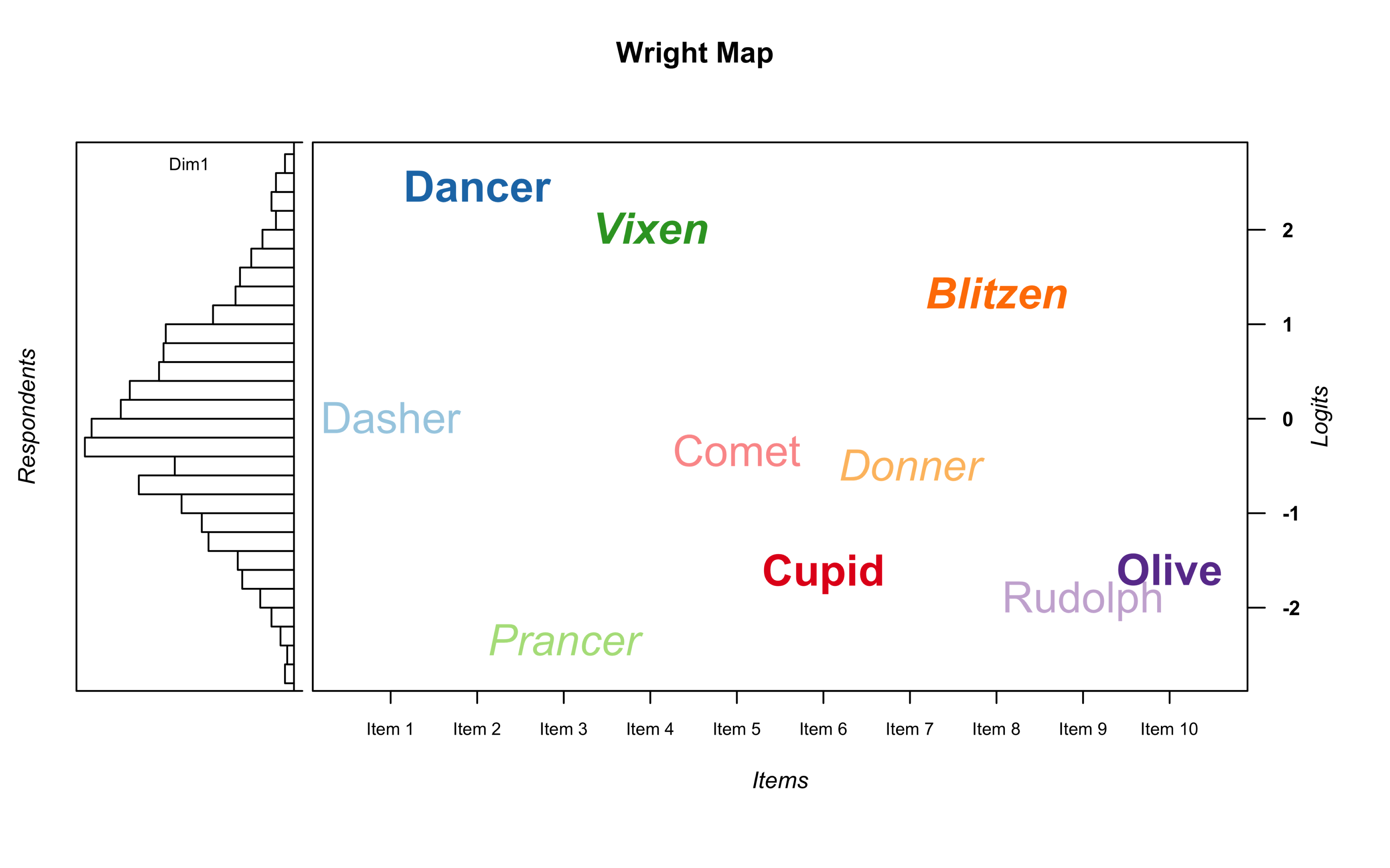
Finally, if you want to go crazy, you can also change the type style using thr.lab.font. This parameter follows the R convention where 1 = plain, 2 = bold, 3 = italic, 4 = bold italic.
For this example, we are going to pass a vector of length 4 with each style. wrightMap will deal with this by repeating it until it matches the number of item difficulties, 10 in this case, so it will produce the following vector: c(1,2,3,4,1,2,3,4,1,2) .
wrightMap(rasch.sim.thetas, rasch.sim.thresholds, show.thr.sym = FALSE
	, thr.lab.text = itemnames, thr.lab.col = itemcolors
	, thr.lab.cex = 1.5, thr.lab.font = c(1:4))